How Much Floor Vibration Can an SEM Tolerate?

Why Does an SEM Care About Floor Vibration at All?

A scanning electron microscope resolves nanometer-scale detail while the floor beneath it moves by micrometers — a mismatch of roughly three orders of magnitude. The two can coexist only because the microscope tolerates a limited amount of floor motion before the image degrades, and that tolerance is exactly what the vendor's installation specification quantifies. "How much floor vibration can an SEM tolerate" therefore has a genuinely numerical answer, and this note gives it.

Two mechanisms convert floor motion into image error. The first is direct relative motion: an SEM builds its image serially, one pixel at a time, so any relative displacement between beam and sample during the raster is written into the image — at high magnification, a few nanometers is enough to blur or serrate an edge. The second is geometric amplification through the column. The sample sits at the end of a long mechanical path, so a support rotation of just one microradian displaces a point one meter up the column by a full micrometer. Floor tilt, not only floor translation, becomes lateral beam-sample error — which is why tall, top-heavy columns are the most vibration-sensitive instruments in a building.

The practical consequence: the tolerance is expressed as a limit on floor velocity as a function of frequency. The sections below give the standard number, show how to measure a real floor against it, and explain the options when the floor fails. For a deeper treatment of the blur mechanisms themselves, see our companion note on vibration isolation for SEM and AFM.

The Number You're Looking For: VC-D, 6.25 μm/s

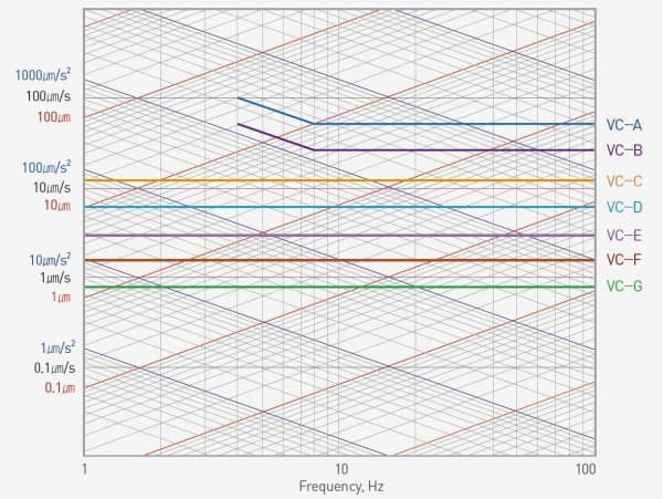
For most floor-standing scanning electron microscopes, the working answer is VC-D: 6.25 μm/s RMS velocity in each one-third-octave band, evaluated from 1 to 80 Hz. The VC (vibration criterion) curves, developed by Colin Gordon and his associates, are the generic vibration classes used worldwide to rate facilities for sensitive instruments, and each step down the ladder halves the allowable velocity.

The rungs that matter for electron microscopy are these.

VC-C — 12.5 μm/s (500 μin/s). Adequate for optical microscopes to 1000x and moderately sensitive electron microscopes working to about 1 μm detail size: entry-level and mid-magnification SEM work.

VC-D — 6.25 μm/s (250 μin/s). Suitable in most instances for demanding equipment, including many electron microscopes (SEMs and TEMs) and e-beam systems, at detail sizes of 0.1–0.3 μm. This is the class most high-resolution SEM installations are designed against.

VC-E — 3.12 μm/s (125 μin/s). A challenging criterion to achieve, assumed adequate for the most demanding sensitive systems — e-beam lithography working at nanometer scales — and cited for the highest-resolution instruments.

Two caveats keep the number honest. First, a VC class is generic guidance, not a contract: the instrument vendor's own site specification is the document a facility must meet, and some ultra-high-resolution columns specify tighter, frequency-dependent limits than any generic class. Second, the criterion is defined per one-third-octave band — a floor can look acceptable in overall RMS yet fail in the single band where an air handler runs.

How Do You Actually Measure Your Floor?

A floor survey that can support an SEM siting decision has four requirements.

Use a seismic-grade sensor. Verifying VC-D means resolving a few micrometers per second of RMS velocity. Seismic-grade velocity sensors — geophones with typical sensitivity of 2.55 V/in/s, about 100.4 V/m/s — read that level directly in the criterion's own units; general-purpose MEMS accelerometers have noise floors well above the signal at low frequency and will report their own noise as floor vibration.

Measure three axes at the actual footprint. Vertical plus two horizontal, at the exact proposed instrument position — not a nearby corridor. Horizontal bands often govern because of the column-lever effect described above, and slab response varies across a single room: mid-span behaves measurably worse than a position near a column line.

Analyze in one-third-octave bands, 1–80 Hz, RMS velocity. This is the form the criterion is written in, so the comparison becomes a band-by-band overlay against the target curve rather than a single number.

Capture the worst realistic window. HVAC on and off, production hours versus night, nearby traffic peaks. A single quiet-hour snapshot is the classic survey error: a floor that passes at 2 a.m. can fail by mid-morning.

The deliverable to insist on is a spectrum overlaid on the target VC curve, stating which bands fail and by how much — because that gap, band by band, is what determines the fix.

How Do You Read the Vendor's Spec Sheet?

SEM site specifications arrive in three formats, and translating between them is where most reading errors happen.

Some vendors simply state a VC class, which maps directly onto the survey described above. Others publish a frequency-dependent limit curve — commonly displacement in micrometers at low frequency and velocity above some corner — and a few specify discrete limits at particular frequencies, reflecting the column's own mechanical resonances. The units matter: for sinusoidal motion, velocity equals 2πf times displacement, so 1 μm of displacement at 1 Hz is about 6.3 μm/s, while the same 1 μm at 10 Hz is 63 μm/s. A constant-displacement limit therefore becomes progressively harder to meet, in velocity terms, as frequency rises — which is exactly why vendors draw curves instead of quoting one number.

Check the statistic as well as the unit. A peak amplitude for a sine equals the RMS value times the square root of two, and comparing a peak-displacement specification against an RMS-velocity survey without converting both is the most common way a compliant floor gets rejected — or a failing one accepted.

Finally, confirm where the specification applies: at the floor under the microscope base, before any isolation. Many columns ship with internal isolators whose effect the vendor has already assumed in the published limit; adding that attenuation twice in your analysis produces false confidence. When in doubt, ask the vendor whether the curve is a bare-floor requirement.

What If Your Floor Exceeds the Limit?

When the survey shows deficits, the options form a ladder. Relocation comes first: a ground-floor slab on grade near a column line, away from mechanical rooms and roads, may pass where an upper-floor mid-span position fails. Most projects, however, do not get to choose the room.

Passive isolation is the traditional next step, and its physics sets its boundary. A pneumatic isolator with a natural frequency of 1.2–3.0 Hz amplifies input near that resonance and isolates effectively only above roughly 5–10 Hz. If the failing bands sit above 10 Hz — pumps, air handlers, machinery harmonics — passive support can close the gap. But building sway, traffic, and slab resonance concentrate their energy below 5 Hz, precisely where a passive mount does nothing or makes matters worse.

Low-frequency deficits call for active vibration isolation: sensors detect the motion and actuators cancel it in real time, in all six degrees of freedom, with isolation effective from 0.5 Hz. For floor-standing SEM and TEM columns, DAEIL SYSTEMS' base-type DVIA-MB platforms carry the instrument on a custom-sized platform — up to 50–80% isolation at 1 Hz and 90% or better from 2 Hz upward over a 0.5–100 Hz active range, with three models spanning payloads from 500 to 6,000 kg. Where the requirement is tighter still, DVIA-ML custom platforms extend the bandwidth to 0.5–200 Hz, reach up to 80–90% attenuation at 1 Hz, and hold magnetic emission below 0.05 μT for field-sensitive electron optics. Behind both stands a track record of more than 1,000 documented installations.

Quick Reference: SEM Floor Vibration Limits at a Glance

The specification. Typical high-resolution floor-standing SEM and TEM: VC-D — 6.25 μm/s RMS per one-third-octave band, 1–80 Hz. Mid-magnification and moderately sensitive electron microscopes: VC-C — 12.5 μm/s. E-beam lithography and the most demanding nanometer-scale systems: VC-E — 3.12 μm/s. Each VC step halves the allowable velocity; the vendor's own site specification always governs over the generic class.

The measurement. Seismic-grade tri-axial velocity sensing at the exact instrument footprint; one-third-octave analysis, 1–80 Hz, RMS velocity; captured across the worst realistic operating window, HVAC and traffic included.

The conversions. Velocity = 2πf × displacement (1 μm at 1 Hz ≈ 6.3 μm/s); sine peak = RMS × √2; confirm whether the vendor curve applies to the bare floor or downstream of built-in isolation.

The fix. Failing bands above roughly 10 Hz: passive isolation can suffice. Failing bands below 5 Hz: only active isolation removes energy there — six-degree-of-freedom control effective from 0.5 Hz, with base-type DVIA-MB platforms carrying floor-standing columns to 6,000 kg and DVIA-ML platforms serving the tightest electron-microscopy requirements.

Kept to those four lines, the answer to the title question is compact: an SEM tolerates roughly 6.25 μm/s of floor vibration in any one-third-octave band — and everything above that number is an isolation problem with a known solution.