Support › Technical Notes › Optical Tables
TECHNICAL NOTE · DVIO OPTICAL TABLES
Large Optical Table Load Analysis: How Much Does a Honeycomb Breadboard Deflect Under 10 Tonnes?
An optical table is judged not by whether it looks sturdy but by how many micrometers it deflects. This note walks through the finite-element verification of a 7 m × 1.5 m DVIO optical table under a 10-tonne load, and explains why the honeycomb core has to be modeled directly rather than approximated.
DAEIL SYSTEMS Engineering6 min read
- Table analyzed
- 7 m × 1.5 m
- Design load margin
- 10 t
- Peak deflection (equipment layout)
- 83 μm
- Safety factor vs. yield
- ≈ 8
1. Why large optical tables need a load analysis
A 7-metre optical table is not a catalog item. Optical benches, collimators, reference flats, and payload jigs weighing several tonnes each sit at specific positions on the top plate, and that layout differs from one customer to the next. The designer has to answer two questions: does the top plate stay within its deflection allowance, and do the structural members keep an adequate margin below the material’s yield strength?
Answering by experience or by adding plate thickness makes the table needlessly heavy; under-designing lets an aligned optical train shift whenever the load changes. For large DVIO configurations, DAEIL SYSTEMS verifies deflection and stress by finite-element analysis before shipment and uses the result to fix design variables such as top- and bottom-skin thickness. This note shows that procedure on a real case.
2. What was analyzed, and how
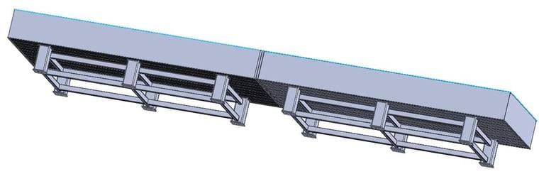
The subject is a 7 m × 1.5 m DVIO configuration: two honeycomb breadboards joined end-to-end on a Rigid Support Table. The customer specified a load margin of at least 10 tonnes; the question was whether the breadboard skins needed to be thickened.
| Item | Detail |
|---|---|
| Configuration | Rigid Support Table + honeycomb breadboards (7 m × 1.5 m) |
| Breadboard skins | 9 mm steel, 3D solid elements |
| Honeycomb core | 0.25 mm steel foil, 2D shell elements |
| Support table | Steel, 3D solid elements |
| Analysis type | Linear static (midas NFX) |
| Boundary condition | Support-table base fixed |
Two load cases were run.
| Case A: Uniform load | Case B: Actual equipment layout | |
|---|---|---|
| Total load | 10 t | ≈ 9.5 t |
| Distribution | Uniform over the entire top plate | Optical bench 2,000 kg · payload 2,000 kg · collimator 3,500 kg · reference flat 1,500 kg, each at its mounting position |
| Application | Pressure load over the top plate | Concentrated loads at the nodes under each footprint |
Case A is the number on the specification sheet; Case B is what the table will actually carry. The total is smaller in B, but a concentrated load placed mid-span between supports can produce a larger local deflection. That is why both cases are checked.
3. What changes when the honeycomb is modeled directly
The usual practice for breadboard analysis is to ignore the internal honeycomb, replace the core with a solid block, and tune an equivalent elastic modulus to match the stiffness. It is fast, but the model cannot tell you how far the core’s real shear behavior departs from the approximation.

In this analysis the 0.25 mm honeycomb foil was meshed directly as 2D shell elements. The cell-wall positions were imprinted onto the skins so that nodes coincide, shell and solid nodes were merged to connect core and skins, and a modal analysis confirmed that the six rigid-body modes separated cleanly — the check that the model is properly connected. To keep the computation tractable, the curved cell profile was linearized; the model converged at roughly 1.3 million degrees of freedom in about 800 seconds.
The difference shows up directly in the results.
| Model | Load case | Peak deflection | Peak stress |
|---|---|---|---|
| Equivalent solid core (conventional) | 10 t uniform | 5 μm | 3 MPa |
| Honeycomb modeled as 2D shells | 10 t uniform | 52 μm | 29 MPa |
| Honeycomb modeled as 2D shells | Actual equipment layout | 83 μm | 28 MPa |
The equivalent-solid model underestimated both deflection and stress by roughly a factor of ten, because it overestimates core stiffness. The absolute values are still small — but a 10× difference is the difference between a safety factor of 80 and a safety factor of 8, and only the latter is a number you can fix a design on.
The equivalent-solid model said 5 μm. The honeycomb-resolved model said 52 μm. Both are “small enough” — but only one of them is the number you sign off a design with.
4. Results: 10 t uniform load vs. real equipment layout
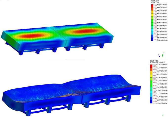
Case A (10 t uniform): peak deflection 52 μm, peak stress 29 MPa. Deflection peaks at mid-span of each breadboard, the classic distribution.
Case B (actual equipment layout): peak deflection 83 μm, peak stress 28 MPa. The total load is lower than in A, but a concentrated 3,500 kg collimator sitting between supports raises the local deflection. Stress stays at the same level as A.
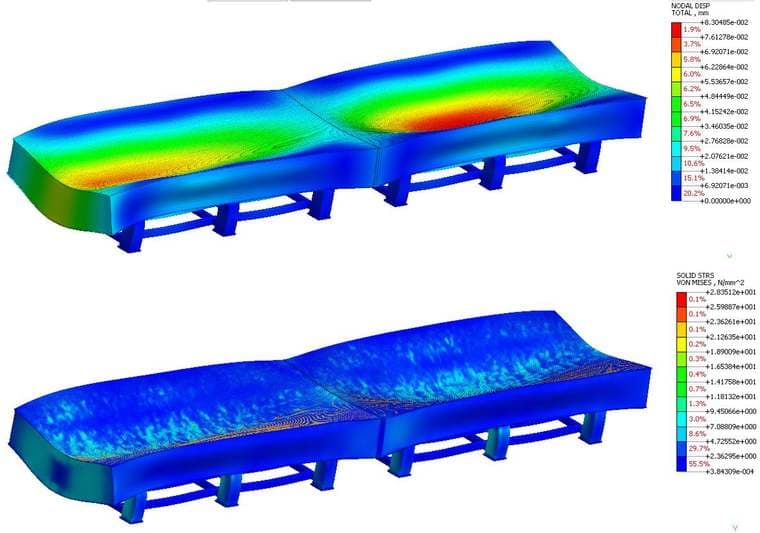
In both cases the peak stress of about 29 MPa gives a safety factor of roughly 8 against the 245 MPa yield strength of general structural steel (SS400). The 83 μm peak deflection is very small relative to the 7 m span and leaves ample margin against the allowance. Linearizing the honeycomb profile may shift the core’s shear stiffness slightly from reality, but at this margin it does not affect the verdict.
5. Design verdict and what it means for your project
The verdict is unambiguous. Under both the 10-tonne uniform load and the real equipment layout, deflection and stress carry ample margin, so no skin-thickness reinforcement is required. Thickening the plates conservatively without analysis would have made the table heavier and more expensive with no gain in performance.
What this case leaves behind is a procedure more than a number. Modeling the honeycomb core directly as 2D shells and connecting the model in the order imprint → node merge → modal check is now DAEIL SYSTEMS’ standard workflow for large-breadboard analysis. If you are planning a large optical table or an unusual load layout, send us the equipment arrangement and load data; we will run the same verification and report deflection and stress before the table is built.
REFERENCES
[1] Gibson, L. J. & Ashby, M. F., Cellular Solids: Structure and Properties, 2nd ed., Cambridge University Press, 1997. — Equivalent stiffness and shear behavior of honeycomb cores
[2] KS D 3503, Rolled steels for general structure (SS400). — 245 MPa yield strength reference