How Active Vibration Cancellation Works: Sensors, DSP, and Actuators

The Signal Chain: Sense, Condition, Compute, Actuate

Every active isolation system executes the same four-stage pipeline thousands of times per second: sense platform motion, condition and amplify the sensor signal, compute a correction digitally, and apply a counter-force. In a DVIA feedback loop, geophone velocity sensors mounted on the isolated platform convert motion into a voltage. An analog front end amplifies and filters that signal before an ADC hands it to the DSP, which runs the control law and drives electromagnetic actuators through a power stage. One deliberate exception: the cleanroom-oriented DVIA-P runs accelerometers and pneumatic servo actuators on the same closed-loop principle, because semiconductor inspection environments are better served by an active-pneumatic force path — the architecture, not the actuator technology, defines the series.

The number that summarizes the whole chain is loop delay. On the fastest DVIA models, the sense-to-force response completes in under 0.5 ms. That figure is not about "reacting quickly" in a colloquial sense; it converts directly into phase. A pure time delay T contributes 360 × f × T degrees of phase lag, so 0.5 ms costs 18 degrees at 100 Hz and 36 degrees at 200 Hz. Phase lag consumes stability margin, stability margin caps usable loop gain, and loop gain is what buys isolation depth. Cutting delay in half does not so much make the system "faster" as buy gain headroom across the entire control band.

Why Low-Frequency Sensing Is the Hard Part

A geophone is a proof mass suspended on a soft spring inside a coil-magnet assembly. Above its natural frequency the mass effectively stands still while the case moves with the platform, so the coil voltage is proportional to velocity — a flat sensitivity of 2.55 V/in/s (about 100.4 V/m/s) in the sensors used on DVIA platforms. Below the natural frequency the physics reverses: the mass increasingly follows the case, relative motion collapses, and output falls at roughly 12 dB per octave. The problem is that the most damaging vibration for metrology — building sway, wind-driven structural motion, slab modes in the 0.5-to-a-few-hertz range — lives exactly where a raw geophone is going deaf.

Recovering that band takes two stages of compensation. Low-noise analog gain first lifts the microvolt-level signal above the noise of the downstream electronics; the DSP then applies an inverse filter that boosts amplitude and corrects phase against the known rolloff, extending usable sensing down to about 0.3 Hz. There is no free lunch: compensation amplifies sensor self-noise along with signal, so the sensor's noise floor ultimately sets how far down the band can be pushed, and the compensation filter's own phase behavior has to be budgeted into the loop design. It is a solvable engineering problem, but it is the reason sub-hertz active control is a specialist discipline rather than a firmware feature.

Feedback and Feedforward: Two Loops, Different Jobs

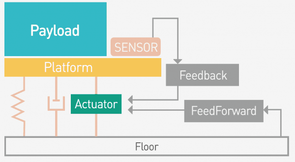
The feedback loop closes around the payload itself. Its geophones measure the residual motion the instrument actually experiences, whatever the source: floor input that leaked through, acoustic pressure on enclosure panels, a stage stepping inside the tool, cable drag. The DSP drives the actuators to null that measurement. Feedback is comprehensive but constrained — it can only act after an error already exists, and its gain is capped by the stability limits discussed below.

The feedforward path starts earlier. Sensors on the floor measure incoming ground vibration before it has propagated through the isolators, and the controller computes a cancelling force in advance, so a large share of the disturbance never registers on the payload at all. Because this path does not feed the platform's own motion back into itself, it carries no stability penalty and its gain can be set aggressively. Its weakness is scope: it cancels only what the floor sensors see, and its accuracy depends on how well the transfer path from floor to payload has been identified and tuned.

Neither loop substitutes for the other. Feedforward takes the predictable ground input off the table; feedback absorbs modeling error plus every disturbance that originates on the platform, which floor sensors cannot observe even in principle. DVIA systems run both concurrently — a practical division of labor, not a redundancy.

Loop Stability: Gain Margin, Phase Margin, and Notch Filters

The isolation delivered by feedback scales with loop gain: disturbances are suppressed roughly by a factor of one plus the loop gain, so the designer wants gain as high as possible across the control band. What prevents infinite gain is phase. Every element in the chain — sensor dynamics, compensation filters, the loop delay itself, actuator response — adds phase lag, and at the frequency where the accumulated lag reaches 180 degrees, a "cancelling" force has rotated into a reinforcing one. If loop gain is still at or above unity there, the system oscillates. Gain margin and phase margin quantify how far the design stays from that cliff.

Real payloads make this harder because they are not rigid bodies. The platform frame, granite mass, and the instrument itself have structural resonances that usually sit inside the control band; at each one, plant gain spikes and phase rotates rapidly, and an untreated loop will sing at exactly those frequencies. The standard remedy is notch filters in the DSP: narrow cuts in loop gain at each structural mode, which let the designer hold high gain everywhere else. This is why tuning against the actual payload matters — a platform engineered for a specific electron-optics column, as in the DVIA-ML program, is stabilized against measured plant dynamics rather than generic assumptions. It is also a quiet argument for digital control: adding a notch is a parameter change, not a soldering iron.

Six Degrees of Freedom: Seeing the Rocking Modes

A floating payload moves in six degrees of freedom: three translations (X, Y, Z) and three rotations (θx, θy, θz). The rotations matter more than intuition suggests. A tall instrument — an electron column is the canonical case — acts as a lever arm that converts a small platform tilt into a large lateral displacement at the top, where the optics are. These rocking modes are among the dominant error sources in SEM and TEM installations.

A single sensor at a single point cannot tell the difference. Pure horizontal translation and rocking about a distant axis produce the same local velocity reading, and a controller acting on that one signal will suppress translation while remaining blind to — or actively feeding — the rotational mode. Genuine 6-DOF control therefore requires an array: multiple sensors whose readings the DSP transforms into six rigid-body modal coordinates, an independent control loop closed on each mode, and a reverse transform that distributes the modal force commands across multiple actuators. DVIA active platforms are built as this kind of MIMO system rather than as six separate single-axis controllers.

The practical consequences surface at installation. Sensor and actuator placement relative to the payload's center of gravity determines how cleanly the modes decouple — which is why site surveys ask for instrument CoG data, and why a heavily asymmetric payload deserves a custom platform rather than a generic one.

What the Chain Delivers — and Where Each DVIA Model Fits

Follow the chain end to end and the datasheet numbers become legible. Active control on DVIA platforms begins at 0.5 Hz and extends to 200 Hz depending on model; the DVIA-ML holds 80–90% isolation at 1 Hz and 90% or better from 2 Hz upward — precisely the band where a passive pneumatic isolator, with a natural frequency of 1.2–3.0 Hz, amplifies rather than isolates and only performs well above roughly 5–10 Hz. Electron optics adds a second-order requirement the chain must respect: the actuators must not become the disturbance, so the DVIA-ML holds magnetic emission below 0.05 μT. Platform capacity scales to 6,000 kg on the DVIA-ML6000, and supported instrument classes cover VC-B through VC-G environments under the VC vibration criteria.

Model selection follows the disturbance problem, not the other way around — from the tabletop DVIA-T to custom DVIA-ML platforms and the active-pneumatic DVIA-P for cleanroom tools. For the model-by-model comparison, including the active-versus-passive decision itself, see our active vibration isolation overview; this note should leave you reading those datasheets as descriptions of a signal chain rather than a list of disconnected numbers.